How one can Make a Chart or Graph in Excel [With Video Tutorial]

Constructing charts and graphs are among the finest methods to visualize knowledge in a transparent and understandable means.

Nevertheless, it is no shock that some individuals get somewhat intimidated by the prospect of poking round in Microsoft Excel.

I assumed I would share a useful video tutorial in addition to some step-by-step directions for anybody on the market who cringes on the considered organizing a spreadsheet full of information right into a chart that really, you realize, means one thing. However earlier than diving in, we should always go over the several types of charts you possibly can create within the software program.

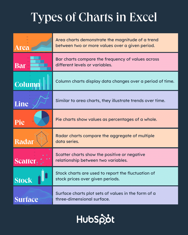
Varieties of Charts in Excel

You may make extra than simply bar or line charts in Microsoft Excel, and once you perceive the makes use of for every, you possibly can draw extra insightful info in your or your staff’s tasks.

The steps you have to construct a chart or graph in Excel are easy, and right here’s a fast walkthrough on the right way to make them.

Obtain Demo Information | Obtain Directions (Mac) | Obtain Directions (PC)

1. Enter your knowledge into Excel.

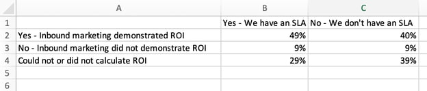
First, you have to enter your knowledge into Excel. You may need exported the information from elsewhere, like a chunk of advertising software program or a survey software. Or perhaps you are inputting it manually.

Within the instance under, in Column A, I’ve an inventory of responses to the query, “Did inbound advertising show ROI?”, and in Columns B, C, and D, I’ve the responses to the query, “Does your organization have a proper sales-marketing settlement?” For instance, Column C, Row 2 illustrates that 49% of individuals with a service degree settlement (SLA) additionally say that inbound advertising demonstrated ROI.

2. Select from the graph and chart choices.

In Excel, your choices for charts and graphs embrace column (or bar) graphs, line graphs, pie graphs, scatter plots, and extra. See how Excel identifies each within the high navigation bar, as depicted under:

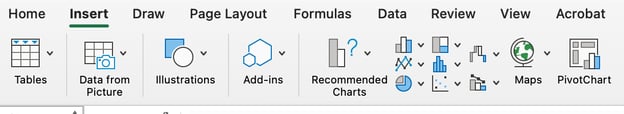
To search out the chart and graph choices, choose Insert.

(For assist determining which kind of chart/graph is greatest for visualizing your knowledge, try our free e book, How one can Use Information Visualization to Win Over Your Viewers.)

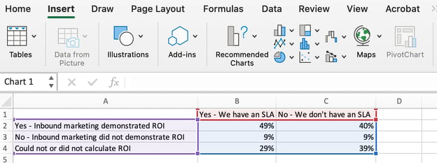
3. Spotlight your knowledge and insert your required graph into the spreadsheet.

On this instance, a bar graph presents the information visually. To make a bar graph, spotlight the information and embrace the titles of the X and Y-axis. Then, go to the Insert tab and click on the column icon within the charts part. Select the graph you would like from the dropdown window that seems.

I picked the primary two dimensional column possibility as a result of I favor the flat bar graphic over the three dimensional look. See the ensuing bar graph under.

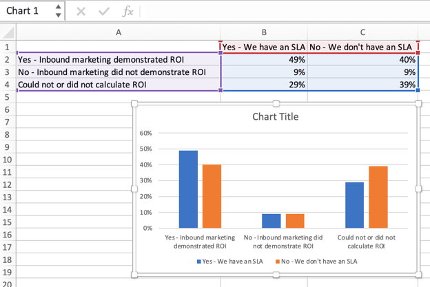
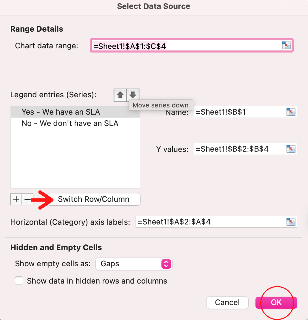
4. Swap the information on every axis, if vital.

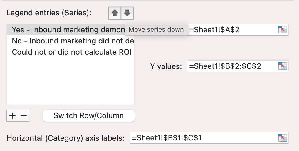
If you wish to swap what seems on the X and Y axis, right-click on the bar graph, click on Choose Information, and click on Swap Row/Column. This can rearrange which axes carry which items of information within the listing proven under. When completed, click on OK on the backside.

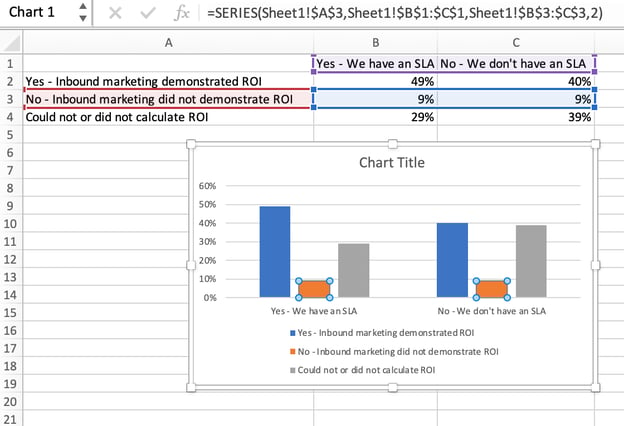
The ensuing graph would appear to be this:

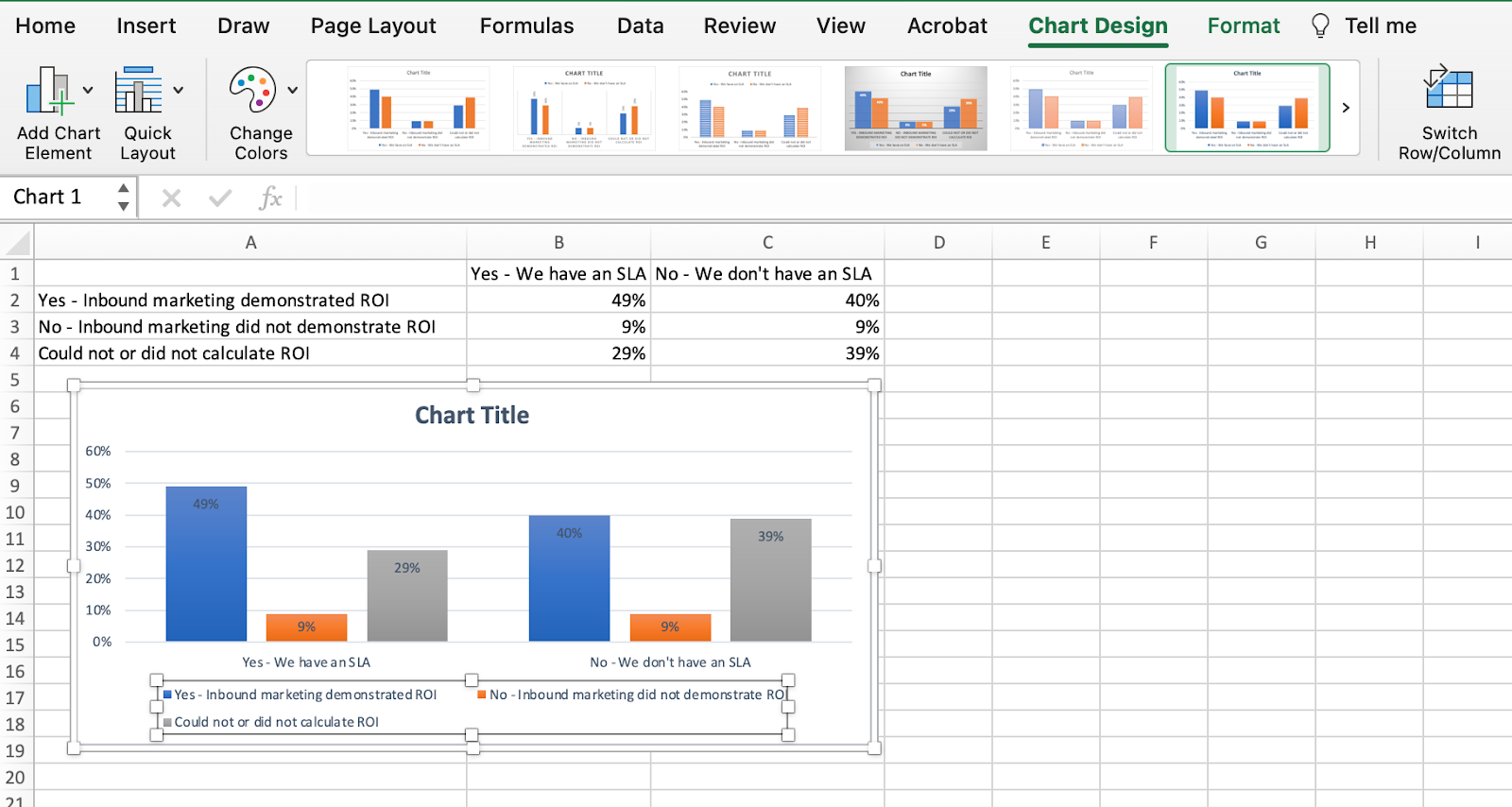
5. Modify your knowledge’s structure and colours.

To vary the labeling structure and legend, click on on the bar graph, then click on the Chart Design tab. Right here, you possibly can select which structure you favor for the chart title, axis titles, and legend. In my instance under, I clicked on the choice that displayed softer bar colours and legends under the chart.

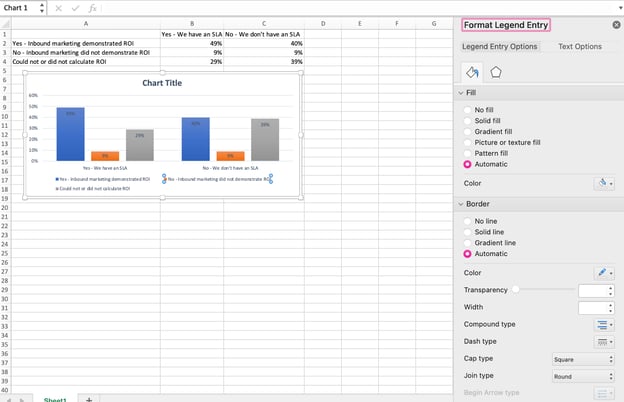
To additional format the legend, click on on it to disclose the Format Legend Entry sidebar, as proven under. Right here, you possibly can change the fill colour of the legend, which is able to change the colour of the columns themselves. To format different elements of your chart, click on on them individually to disclose a corresponding Format window.

6. Change the scale of your chart’s legend and axis labels.

Once you first make a graph in Excel, the scale of your axis and legend labels is likely to be small, relying on the graph or chart you select (bar, pie, line, and so on.) As soon as you have created your chart, you may need to beef up these labels so that they’re legible.

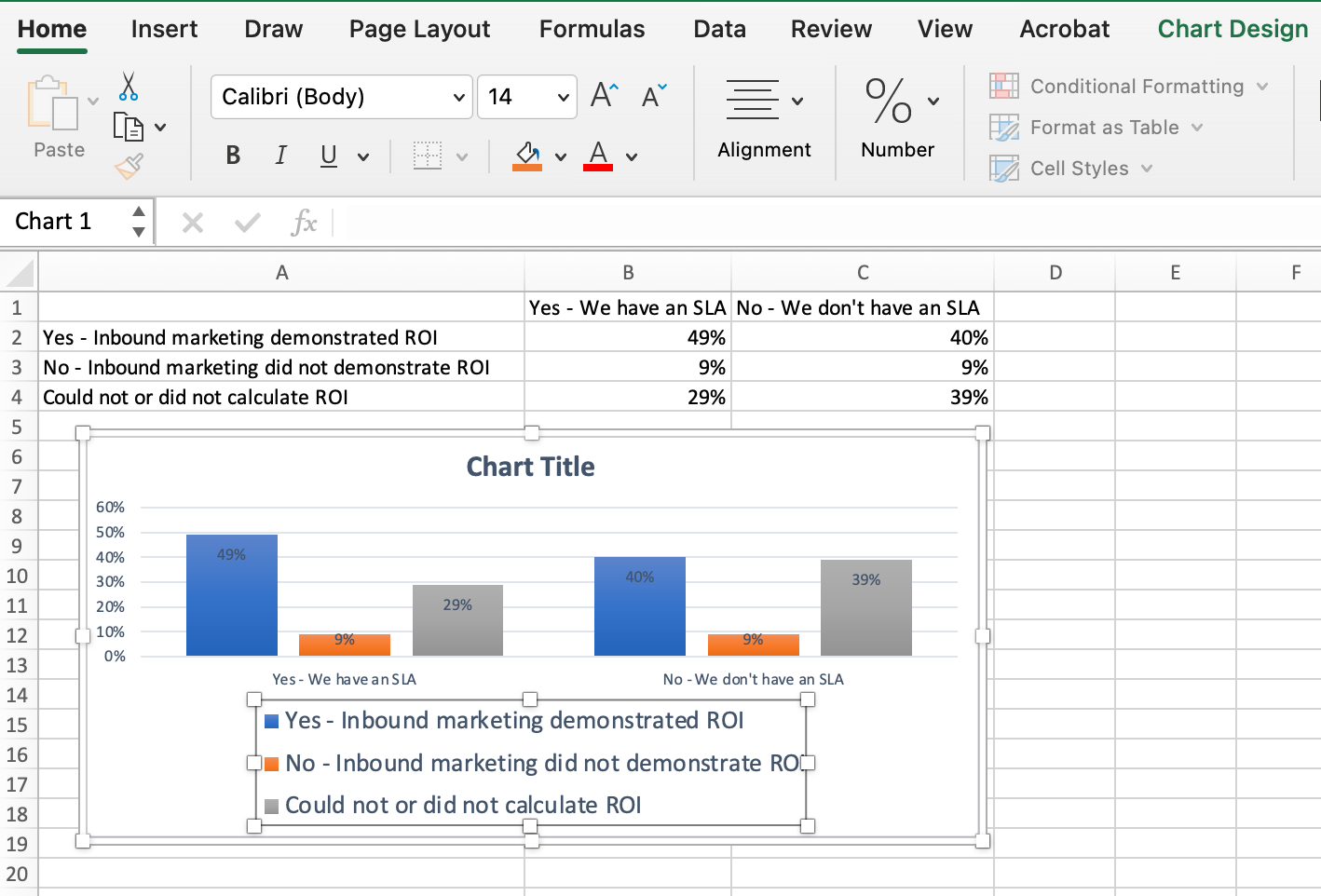
To extend the scale of your graph’s labels, click on on them individually and, as a substitute of unveiling a brand new Format window, click on again into the House tab within the high navigation bar of Excel. Then, use the font sort and dimension dropdown fields to increase or shrink your chart’s legend and axis labels to your liking.

7. Change the Y-axis measurement choices if desired.

To vary the kind of measurement proven on the Y axis, click on on the Y-axis percentages in your chart to disclose the Format Axis window. Right here, you possibly can determine if you wish to show items situated on the Axis Choices tab, or if you wish to change whether or not the Y-axis exhibits percentages to 2 decimal locations or no decimal locations.

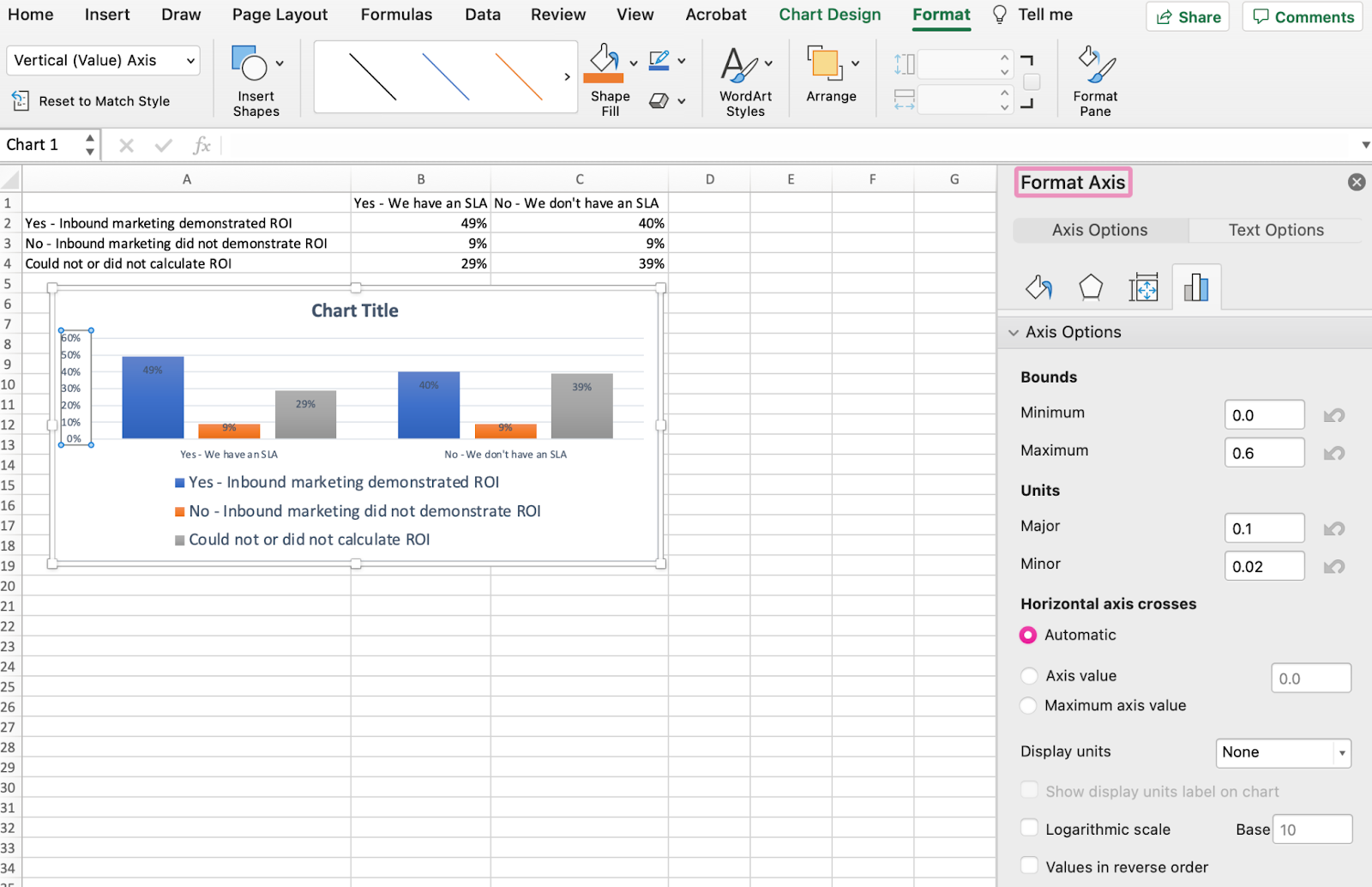
As a result of my graph robotically units the Y axis’s most share to 60%, you would possibly need to change it manually to 100% to signify my knowledge on a common scale. To take action, you possibly can choose the Most possibility — two fields down beneath Bounds within the Format Axis window — and alter the worth from 0.6 to at least one.

The ensuing graph will appear to be the one under (On this instance, the font dimension of the Y-axis has been elevated through the House tab with the intention to see the distinction):

8. Reorder your knowledge, if desired.

To type the information so the respondents’ solutions seem in reverse order, right-click in your graph and click on Choose Information to disclose the identical choices window you referred to as up in Step 3 above. This time, arrow up and right down to reverse the order of your knowledge on the chart.

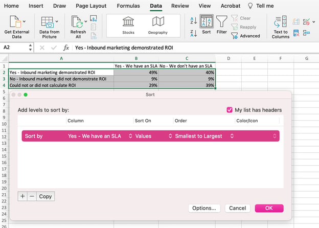
In case you have greater than two strains of information to regulate, you too can rearrange them in ascending or descending order. To do that, spotlight your entire knowledge within the cells above your chart, click on Information and choose Type, as proven under. Relying in your desire, you possibly can select to type based mostly on smallest to largest, or vice versa.

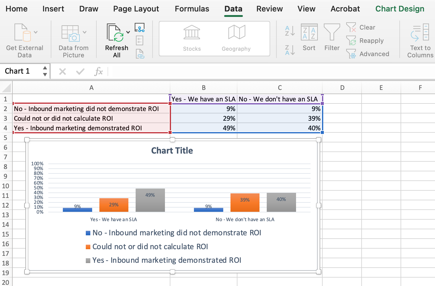
The ensuing graph would appear to be this:

9. Title your graph.

Now comes the enjoyable and simple half: naming your graph. By now, you may need already found out how to do that. Here is a easy clarifier.

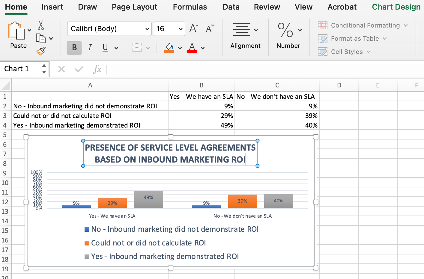
Proper after making your chart, the title that seems will seemingly be “Chart Title,” or one thing comparable relying on the model of Excel you are utilizing. To vary this label, click on on “Chart Title” to disclose a typing cursor. You’ll be able to then freely customise your chart’s title.

When you could have a title you want, click on House on the highest navigation bar, and use the font formatting choices to offer your title the emphasis it deserves. See these choices and my ultimate graph under:

10. Export your graph or chart.

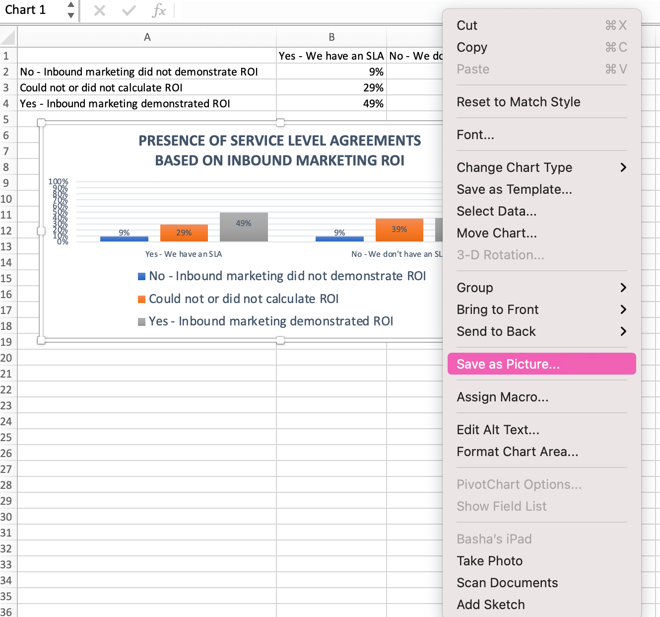
As soon as your chart or graph is precisely the best way you need it, it can save you it as a picture with out screenshotting it within the spreadsheet. This methodology offers you a clear picture of your chart that may be inserted right into a PowerPoint presentation, Canva doc, or some other visible template.

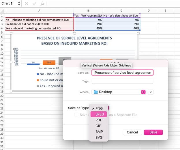
To save lots of your Excel graph as a photograph, right-click on the graph and choose Save as Image.

Within the dialogue field, title the picture of your graph, select the place to reserve it in your laptop, and select the file sort you’d like to reserve it as. On this instance, it’s saved as a JPEG to a desktop folder. Lastly, click on Save.

You’ll have a transparent picture of your graph or chart that you may add to any visible design.

Visualize Information Like A Professional

That was fairly straightforward, proper? With this step-by-step tutorial, you’ll be capable of shortly create charts and graphs that visualize essentially the most difficult knowledge. Strive utilizing this identical tutorial with totally different graph sorts like a pie chart or line graph to see what format tells the story of your knowledge greatest.

Editor’s observe: This submit was initially printed in June 2018 and has been up to date for comprehensiveness.