


Typically, Excel appears too good to be true. All I’ve to do is enter a components, and just about something I would ever have to do manually may be achieved routinely.
Must merge two sheets with comparable information? Excel can do it.
Must do simple arithmetic? Excel can do it.
Want to mix data in a number of cells? Excel can do it.
On this put up, I’ll go over one of the best suggestions, tips, and shortcuts you should use proper now to take your Excel sport to the subsequent stage. No superior Excel information required.
![Download 10 Excel Templates for Marketers [Free Kit]](https://no-cache.hubspot.com/cta/default/53/9ff7a4fe-5293-496c-acca-566bc6e73f42.png)
What’s Excel?
Microsoft Excel is highly effective information visualization and evaluation software program, which makes use of spreadsheets to retailer, manage, and monitor information units with formulation and capabilities. Excel is utilized by entrepreneurs, accountants, information analysts, and different professionals. It is a part of the Microsoft Workplace suite of merchandise. Options embrace Google Sheets and Numbers.
Discover extra Excel alternate options right here.
What’s Excel used for?
Excel is used to retailer, analyze, and report on giant quantities of knowledge. It’s typically utilized by accounting groups for monetary evaluation, however can be utilized by any skilled to handle lengthy and unwieldy datasets. Examples of Excel purposes embrace stability sheets, budgets, or editorial calendars.
Excel is primarily used for creating monetary paperwork due to its sturdy computational powers. You’ll typically discover the software program in accounting places of work and groups as a result of it permits accountants to routinely see sums, averages, and totals. With Excel, they’ll simply make sense of their enterprise’ information.
Whereas Excel is primarily often known as an accounting software, professionals in any area can use its options and formulation — particularly entrepreneurs — as a result of it may be used for monitoring any sort of knowledge. It removes the necessity to spend hours and hours counting cells or copying and pasting efficiency numbers. Excel sometimes has a shortcut or fast repair that hastens the method.
You can too obtain Excel templates beneath for your entire advertising and marketing wants.
After you obtain the templates, it’s time to begin utilizing the software program. Let’s cowl the fundamentals first.
Excel Fundamentals
In the event you’re simply beginning out with Excel, there are a couple of primary instructions that we advise you turn out to be accustomed to. These are issues like:
- Creating a brand new spreadsheet from scratch.
- Executing primary computations like including, subtracting, multiplying, and dividing.
- Writing and formatting column textual content and titles.
- Utilizing Excel’s auto-fill options.
- Including or deleting single columns, rows, and spreadsheets. (Under, we’ll get into the right way to add issues like a number of columns and rows.)
- Preserving column and row titles seen as you scroll previous them in a spreadsheet, in order that you understand what information you are filling as you progress additional down the doc.
- Sorting your information in alphabetical order.
Let’s discover a couple of of those extra in-depth.
For example, why does auto-fill matter?
If in case you have any primary Excel information, it’s doubtless you already know this fast trick. However to cowl our bases, enable me to indicate you the glory of autofill. This allows you to shortly fill adjoining cells with a number of forms of information, together with values, collection, and formulation.
There are a number of methods to deploy this characteristic, however the fill deal with is among the many best. Choose the cells you wish to be the supply, find the fill deal with within the lower-right nook of the cell, and both drag the fill deal with to cowl cells you wish to fill or simply double click on:
 Equally, sorting is a crucial characteristic you may wish to know when organizing your information in Excel.
Typically you might have a listing of knowledge that has no group in anyway. Possibly you exported a listing of your advertising and marketing contacts or weblog posts. Regardless of the case could also be, Excel’s kind characteristic will assist you to alphabetize any listing.
Click on on the info within the column you wish to kind. Then click on on the “Knowledge” tab in your toolbar and search for the “Type” choice on the left. If the “A” is on prime of the “Z,” you may simply click on on that button as soon as. If the “Z” is on prime of the “A,” click on on the button twice. When the “A” is on prime of the “Z,” which means your listing will likely be sorted in alphabetical order. Nonetheless, when the “Z” is on prime of the “A,” which means your listing will likely be sorted in reverse alphabetical order.
Let’s discover extra of the fundamentals of Excel (together with superior options) subsequent.
How one can Use Excel
To make use of Excel, you solely have to enter the info into the rows and columns. And then you definitely’ll use formulation and capabilities to show that information into insights.
We‘re going to go over one of the best formulation and capabilities you should know. However first, let’s check out the forms of paperwork you may create utilizing the software program. That approach, you may have an overarching understanding of how you should use Excel in your day-to-day.
Paperwork You Can Create in Excel
Unsure how one can truly use Excel in your workforce? Here’s a listing of paperwork you may create:
- Earnings Statements: You need to use an Excel spreadsheet to trace an organization’s gross sales exercise and monetary well being.
- Steadiness Sheets: Steadiness sheets are among the many commonest forms of paperwork you may create with Excel. It lets you get a holistic view of an organization’s monetary standing.
- Calendar: You possibly can simply create a spreadsheet month-to-month calendar to trace occasions or different date-sensitive data.
Listed here are some paperwork you may create particularly for entrepreneurs.
That is solely a small sampling of the forms of advertising and marketing and enterprise paperwork you may create in Excel. We’ve created an in depth listing of Excel templates you should use proper now for advertising and marketing, invoicing, venture administration, budgeting, and extra.
Within the spirit of working extra effectively and avoiding tedious, handbook work, listed here are a couple of Excel formulation and capabilities you’ll have to know.
Excel Formulation
It’s simple to get overwhelmed by the big selection of Excel formulation that you should use to make sense out of your information. In the event you’re simply getting began utilizing Excel, you may depend on the next formulation to hold out some advanced capabilities — with out including to the complexity of your studying path.
- Equal signal: Earlier than creating any components, you’ll want to put in writing an equal signal (=) within the cell the place you need the consequence to seem.
- Addition: So as to add the values of two or extra cells, use the + signal. Instance: =C5+D3.
- Subtraction: To subtract the values of two or extra cells, use the – signal. Instance: =C5-D3.
- Multiplication: To multiply the values of two or extra cells, use the * signal. Instance: =C5*D3.
- Division: To divide the values of two or extra cells, use the / signal. Instance: =C5/D3.
Placing all of those collectively, you may create a components that provides, subtracts, multiplies, and divides multi functional cell. Instance: =(C5-D3)/((A5+B6)*3).
For extra advanced formulation, you’ll want to make use of parentheses across the expressions to keep away from by accident utilizing the PEMDAS order of operations. Take into account that you should use plain numbers in your formulation.
Excel Capabilities
Excel capabilities automate a few of the duties you’ll use in a typical components. For example, as a substitute of utilizing the + signal so as to add up a variety of cells, you’d use the SUM perform. Let’s have a look at a couple of extra capabilities that may assist automate calculations and duties.
- SUM: The SUM perform routinely provides up a variety of cells or numbers. To finish a sum, you’ll enter the beginning cell and the ultimate cell with a colon in between. Right here’s what that appears like: SUM(Cell1:Cell2). Instance: =SUM(C5:C30).
- AVERAGE: The AVERAGE perform averages out the values of a variety of cells. The syntax is similar because the SUM perform: AVERAGE(Cell1:Cell2). Instance: =AVERAGE(C5:C30).
- IF: The IF perform lets you return values based mostly on a logical check. The syntax is as follows: IF(logical_test, value_if_true, [value_if_false]). Instance: =IF(A2>B2,“Over Price range”,“OK”).
- VLOOKUP: The VLOOKUP perform helps you seek for something in your sheet’s rows. The syntax is: VLOOKUP(lookup worth, desk array, column quantity, Approximate match (TRUE) or Actual match (FALSE)). Instance: =VLOOKUP([@Attorney],tbl_Attorneys,4,FALSE).
- INDEX: The INDEX perform returns a worth from inside a variety. The syntax is as follows: INDEX(array, row_num, [column_num]).
- MATCH: The MATCH perform seems for a sure merchandise in a variety of cells and returns the place of that merchandise. It may be utilized in tandem with the INDEX perform. The syntax is: MATCH(lookup_value, lookup_array, [match_type]).
- COUNTIF: The COUNTIF perform returns the variety of cells that meet a sure standards or have a sure worth. The syntax is: COUNTIF(vary, standards). Instance: =COUNTIF(A2:A5,“London”).
Okay, able to get into the nitty-gritty? Let‘s get to it. (And to all of the Harry Potter followers on the market … you’re welcome upfront.)
Excel Suggestions
- Use Pivot tables to acknowledge and make sense of knowledge.
- Add multiple row or column.
- Use filters to simplify your information.
- Take away duplicate information factors or units.
- Transpose rows into columns.
- Break up up textual content data between columns.
- Use these formulation for easy calculations.
- Get the common of numbers in your cells.
- Use conditional formatting to make cells routinely change coloration based mostly on information.
- Use IF Excel components to automate sure Excel capabilities.
- Use greenback indicators to maintain one cell’s components the identical no matter the place it strikes.
- Use the VLOOKUP perform to drag information from one space of a sheet to a different.
- Use INDEX and MATCH formulation to drag information from horizontal columns.
- Use the COUNTIF perform to make Excel rely phrases or numbers in any vary of cells.
- Mix cells utilizing ampersand.
- Add checkboxes.
- Hyperlink a cell to an internet site.
- Add drop-down menus.
- Use the format painter.
- Create tables with information.
- Use tables to conduct a what-if evaluation.
- Make formulation simpler to grasp with named ranges.
- Group information to enhance group.
- Use Discover & Choose to streamline formatting.
- Defend your work.
- Create customized quantity codecs.
- Customise the Excel ribbon.
- Enhance visible presentation with textual content wrapping.
- Add emojis.
Observe: Among the GIFs and visuals are from a earlier model of Excel. When relevant, the copy has been up to date to offer instruction for customers of each newer and older Excel variations.
1. Use Pivot tables to acknowledge and make sense of knowledge.
Pivot tables are used to reorganize information in a spreadsheet. They gained‘t change the info that you’ve, however they’ll sum up values and evaluate totally different data in your spreadsheet, relying on what you’d like them to do.
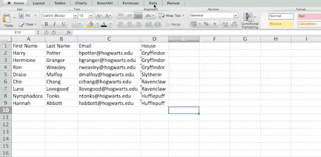
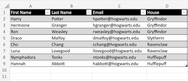
Let‘s check out an instance. Let’s say I need to try how many individuals are in every home at Hogwarts. You could be considering that I haven’t got an excessive amount of information, however for longer information units, this may turn out to be useful.
To create the Pivot Desk, I am going to Knowledge > Pivot Desk. In the event you’re utilizing the newest model of Excel, you’d go to Insert > Pivot Desk. Excel will routinely populate your Pivot Desk, however you may all the time change across the order of the info. Then, you may have 4 choices to select from.
- Report Filter: This lets you solely have a look at sure rows in your dataset. For instance, if I wished to create a filter by home, I might select to solely embrace college students in Gryffindor as a substitute of all college students.
- Column Labels: These can be your headers within the dataset.
- Row Labels: These could possibly be your rows within the dataset. Each Row and Column labels can comprise information out of your columns (e.g. First Title may be dragged to both the Row or Column label — it simply is determined by the way you wish to see the info.)
- Worth: This part lets you have a look at your information otherwise. As a substitute of simply pulling in any numeric worth, you may sum, rely, common, max, min, rely numbers, or do a couple of different manipulations together with your information. In truth, by default, while you drag a area to Worth, it all the time does a rely.
Since I wish to rely the variety of college students in every home, I will go to the Pivot desk builder and drag the Home column to each the Row Labels and the Values. It will sum up the variety of college students related to every home.
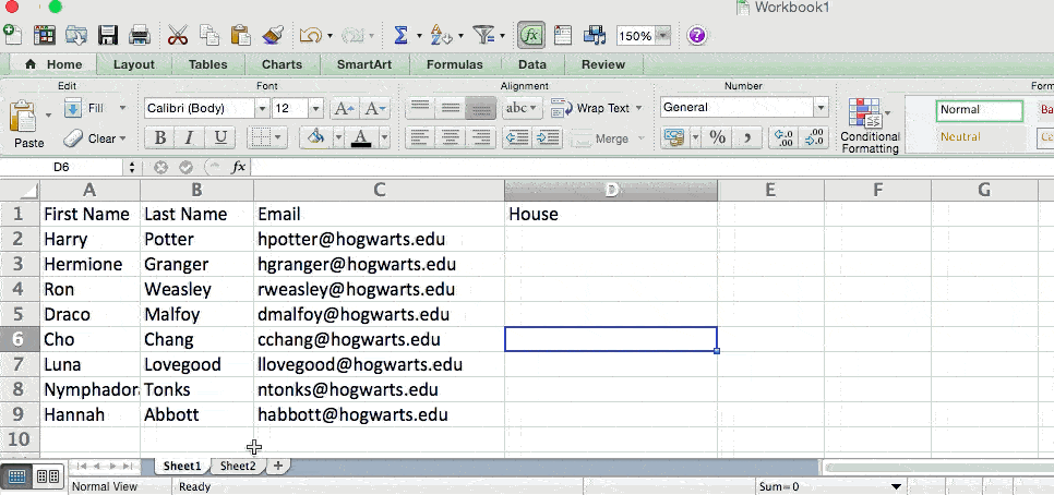
2. Add multiple row or column.
As you mess around together with your information, you would possibly discover you‘re consistently needing so as to add extra rows and columns. Typically, it’s possible you’ll even want so as to add a whole lot of rows. Doing this one-by-one can be tremendous tedious. Fortunately, there’s all the time a neater approach.
So as to add a number of rows or columns in a spreadsheet, spotlight the identical variety of preexisting rows or columns that you just wish to add. Then, right-click and choose “Insert.”
Within the instance beneath, I wish to add a further three rows. By highlighting three rows after which clicking insert, I can add a further three clean rows into my spreadsheet shortly and simply.
3. Use filters to simplify your information.
If you‘re taking a look at very giant information units, you don’t normally have to be taking a look at each single row on the similar time. Typically, you solely wish to have a look at information that match into sure standards.
That is the place filters are available.
Filters permit you to pare down your information to solely have a look at sure rows at one time. In Excel, a filter may be added to every column in your information — and from there, you may then select which cells you wish to view directly.
Let‘s check out the instance beneath. Add a filter by clicking the Knowledge tab and deciding on “Filter.” Clicking the arrow subsequent to the column headers and also you’ll be capable of select whether or not you need your information to be organized in ascending or descending order, in addition to which particular rows you wish to present.
In my Harry Potter instance, to illustrate I solely wish to see the scholars in Gryffindor. By deciding on the Gryffindor filter, the opposite rows disappear.
 Professional Tip: Copy and paste the values within the spreadsheet when a Filter is on to do further evaluation in one other spreadsheet.
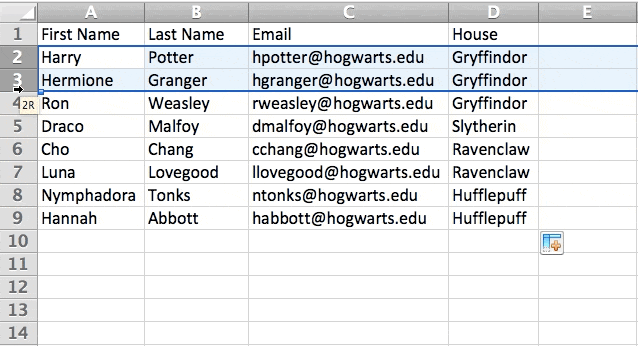
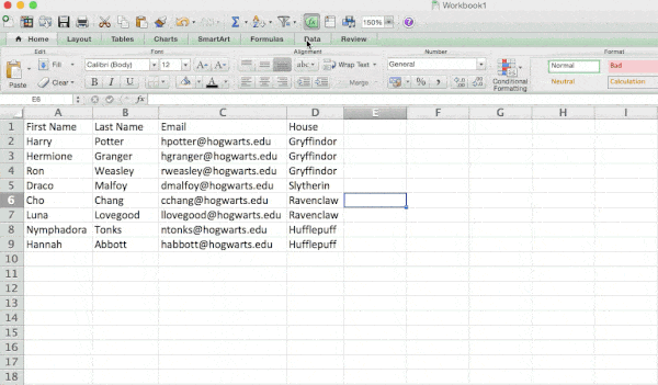
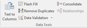
4. Take away duplicate information factors or units.
Bigger information units are likely to have duplicate content material. You will have a listing of a number of contacts in an organization and solely wish to see the variety of corporations you may have. In conditions like this, eradicating the duplicates is available in fairly helpful.
To take away your duplicates, spotlight the row or column that you just wish to take away duplicates of. Then, go to the Knowledge tab and choose “Take away Duplicates” (which is beneath the Instruments subheader within the older model of Excel). A pop-up will seem to substantiate which information you wish to work with. Choose “Take away Duplicates,” and also you’re good to go.
You can too use this characteristic to take away a whole row based mostly on a replica column worth. So you probably have three rows with Harry Potter’s data and also you solely have to see one, then you may choose the entire dataset after which take away duplicates based mostly on electronic mail. Your ensuing listing can have solely distinctive names with none duplicates.
5. Transpose rows into columns.
When you may have rows of knowledge in your spreadsheet, you would possibly resolve you truly wish to remodel the gadgets in a kind of rows into columns (or vice versa). It might take a variety of time to repeat and paste every particular person header — however what the transpose characteristic lets you do is solely transfer your row information into columns, or the opposite approach round.
Begin by highlighting the column that you just wish to transpose into rows. Proper-click it, after which choose “Copy.” Subsequent, choose the cells in your spreadsheet the place you need your first row or column to start. Proper-click on the cell, after which choose “Paste Particular.” A module will seem — on the backside, you may see an choice to transpose. Examine that field and choose OK. Your column will now be transferred to a row or vice-versa.
On newer variations of Excel, a drop-down will seem as a substitute of a pop-up.

6. Break up up textual content data between columns.
What if you wish to cut up out data that‘s in a single cell into two totally different cells? For instance, possibly you wish to pull out somebody’s firm title by their electronic mail handle. Or maybe you wish to separate somebody’s full title into a primary and final title on your electronic mail advertising and marketing templates.
Due to Excel, each are attainable. First, spotlight the column that you just wish to cut up up. Subsequent, go to the Knowledge tab and choose “Textual content to Columns.” A module will seem with further data.
First, you should choose both “Delimited” or “Mounted Width.”
- “Delimited” means you wish to break up the column based mostly on characters resembling commas, areas, or tabs.
- “Mounted Width” means you wish to choose the precise location on all of the columns that you really want the cut up to happen.
Within the instance case beneath, let’s choose “Delimited” so we will separate the total title into first title and final title.
Then, it‘s time to decide on the Delimiters. This could possibly be a tab, semi-colon, comma, area, or one thing else. (“One thing else” could possibly be the “@” signal utilized in an electronic mail handle, for instance.) In our instance, let’s select the area. Excel will then present you a preview of what your new columns will seem like.
If you‘re proud of the preview, press “Subsequent.” This web page will permit you to choose Superior Codecs should you select to. If you’re achieved, click on “End.”
7. Use formulation for easy calculations.
Along with doing fairly advanced calculations, Excel will help you do easy arithmetic like including, subtracting, multiplying, or dividing any of your information.
- So as to add, use the + signal.
- To subtract, use the – signal.
- To multiply, use the * signal.
- To divide, use the / signal.
You can too use parentheses to make sure sure calculations are achieved first. Within the instance beneath (10+10*10), the second and third 10 had been multiplied collectively earlier than including the extra 10. Nonetheless, if we made it (10+10)*10, the primary and second 10 can be added collectively first.
8. Get the common of numbers in your cells.
If you need the common of a set of numbers, you should use the components =AVERAGE(Cell1:Cell2). If you wish to sum up a column of numbers, you should use the components =SUM(Cell1:Cell2).
9. Use conditional formatting to make cells routinely change coloration based mostly on information.
Conditional formatting lets you change a cell’s coloration based mostly on the knowledge throughout the cell. For instance, if you wish to flag sure numbers which can be above common or within the prime 10% of the info in your spreadsheet, you are able to do that. If you wish to coloration code commonalities between totally different rows in Excel, you are able to do that. It will assist you to shortly see data that’s vital to you.
To get began, spotlight the group of cells you wish to use conditional formatting on. Then, select “Conditional Formatting” from the House menu and choose your logic from the dropdown. (You can too create your individual rule if you’d like one thing totally different.) A window will pop up that prompts you to offer extra details about your formatting rule. Choose “OK” while you’re achieved, and it is best to see your outcomes routinely seem.
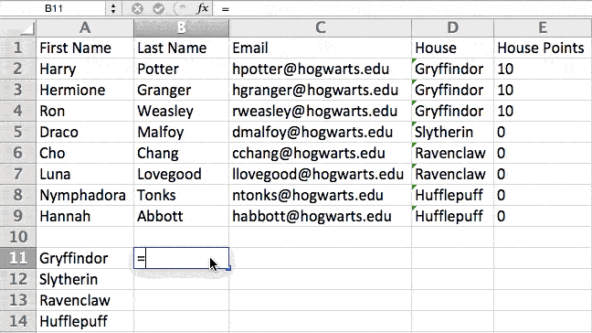
10. Use the IF Excel components to automate sure Excel capabilities.
Typically, we do not wish to rely the variety of instances a worth seems. As a substitute, we wish to enter totally different data right into a cell if there’s a corresponding cell with that data.
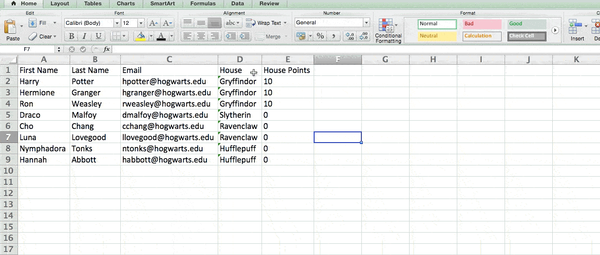
For instance, within the scenario beneath, I wish to award ten factors to everybody who belongs within the Gryffindor home. As a substitute of manually typing in 10‘s subsequent to every Gryffindor pupil’s title, I can use the IF Excel components to say that if the coed is in Gryffindor, then they need to get ten factors.
The components is: IF(logical_test, value_if_true, [value_if_false])
Instance Proven Under: =IF(D2=“Gryffindor”,“10”,“0”)
Generally phrases, the components can be IF(Logical Take a look at, worth of true, worth of false). Let’s dig into every of those variables.
- Logical_Test: The logical check is the “IF” a part of the assertion. On this case, the logic is D2=“Gryffindor” as a result of we wish to make it possible for the cell corresponding with the coed says “Gryffindor.” Be certain that to place Gryffindor in citation marks right here.
- Value_if_True: That is what we would like the cell to indicate if the worth is true. On this case, we would like the cell to indicate “10” to point that the coed was awarded the ten factors. Solely use citation marks if you’d like the consequence to be textual content as a substitute of a quantity.
- Value_if_False: That is what we would like the cell to indicate if the worth is fake. On this case, for any pupil not in Gryffindor, we would like the cell to indicate “0”. Solely use citation marks if you’d like the consequence to be textual content as a substitute of a quantity.
Observe: Within the instance above, I awarded 10 factors to everybody in Gryffindor. If I later wished to sum the overall variety of factors, I wouldn‘t be capable of as a result of the ten’s are in quotes, thus making them textual content and never a quantity that Excel can sum.
The actual energy of the IF perform comes while you string a number of IF statements
Ranges are one technique to section your information for higher evaluation. For instance, you may categorize information into values which can be lower than 10, 11 to 50, or 51 to 100. Here is how that appears in follow:
=IF(B3<11,“10 or much less”,IF(B3<51,“11 to 50”,IF(B3<100,“51 to 100”)))
It may take some trial-and-error, however upon getting the grasp of it, IF formulation will turn out to be your new Excel greatest good friend.
11. Use greenback indicators to maintain one cell’s components the identical no matter the place it strikes.
Have you ever ever seen a greenback sign up an Excel components? When utilized in a components, it is not representing an American greenback; as a substitute, it makes positive that the precise column and row are held the identical even should you copy the identical components in adjoining rows.
You see, a cell reference — while you check with cell A5 from cell C5, for instance — is relative by default. In that case, you‘re truly referring to a cell that’s 5 columns to the left (C minus A) and in the identical row (5). That is referred to as a relative components. If you copy a relative components from one cell to a different, it‘ll regulate the values within the components based mostly on the place it’s moved. However typically, we would like these values to remain the identical irrespective of whether or not they’re moved round or not — and we will do this by turning the components into an absolute components.
To alter the relative components (=A5+C5) into an absolute components, we would precede the row and column values by greenback indicators, like this: (=$A$5+$C$5). (Study extra on Microsoft Workplace’s help web page right here.)
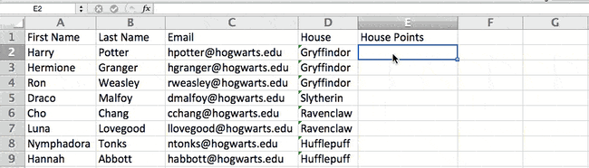
12. Use the VLOOKUP perform to drag information from one space of a sheet to a different.
Have you ever ever had two units of knowledge on two totally different spreadsheets that you just wish to mix right into a single spreadsheet?
For instance, you might need a listing of individuals‘s names subsequent to their electronic mail addresses in a single spreadsheet, and a listing of those self same individuals’s electronic mail addresses subsequent to their firm names within the different — however you need the names, electronic mail addresses, and firm names of these individuals to seem in a single place.
I’ve to mix information units like this so much — and after I do, the VLOOKUP is my go-to components.
Earlier than you employ the components, although, be completely positive that you’ve at the very least one column that seems identically in each locations. Scour your information units to ensure the column of knowledge you are utilizing to mix your data is strictly the identical, together with no further areas.
The components: =VLOOKUP(lookup worth, desk array, column quantity, Approximate match (TRUE) or Actual match (FALSE))
The components with variables from our instance beneath: =VLOOKUP(C2,Sheet2!A:B,2,FALSE)
On this components, there are a number of variables. The next is true while you wish to mix data in Sheet 1 and Sheet 2 onto Sheet 1.
- Lookup Worth: That is the an identical worth you may have in each spreadsheets. Select the primary worth in your first spreadsheet. Within the instance that follows, this implies the primary electronic mail handle on the listing, or cell 2 (C2).
- Desk Array: The desk array is the vary of columns on Sheet 2 you‘re going to drag your information from, together with the column of knowledge an identical to your lookup worth (in our instance, electronic mail addresses) in Sheet 1 in addition to the column of knowledge you’re attempting to repeat to Sheet 1. In our instance, that is “Sheet2!A:B.” “A” means Column A in Sheet 2, which is the column in Sheet 2 the place the info an identical to our lookup worth (electronic mail) in Sheet 1 is listed. The “B” means Column B, which comprises the knowledge that is solely accessible in Sheet 2 that you just wish to translate to Sheet 1.
- Column Quantity: This tells Excel which column the brand new information you wish to copy to Sheet 1 is positioned in. In our instance, this might be the column that “Home” is positioned in. “Home” is the second column in our vary of columns (desk array), so our column quantity is 2. [Note: Your range can be more than two columns. For example, if there are three columns on Sheet 2 — Email, Age, and House — and you still want to bring House onto Sheet 1, you can still use a VLOOKUP. You just need to change the “2” to a “3” so it pulls back the value in the third column: =VLOOKUP(C2:Sheet2!A:C,3,false).]
- Approximate Match (TRUE) or Actual Match (FALSE): Use FALSE to make sure you pull in solely precise worth matches. In the event you use TRUE, the perform will pull in approximate matches.
Within the instance beneath, Sheet 1 and Sheet 2 comprise lists describing totally different details about the identical individuals, and the widespread thread between the 2 is their electronic mail addresses. For instance we wish to mix each datasets so that each one the home data from Sheet 2 interprets over to Sheet 1.
So once we sort within the components =VLOOKUP(C2,Sheet2!A:B,2,FALSE), we convey all the home information into Sheet 1.
Take into account that VLOOKUP will solely pull again values from the second sheet which can be to the best of the column containing your an identical information. This could result in some limitations, which is why some individuals desire to make use of the INDEX and MATCH capabilities as a substitute.
13. Use INDEX and MATCH formulation to drag information from horizontal columns.
Like VLOOKUP, the INDEX and MATCH capabilities pull in information from one other dataset into one central location. Listed here are the principle variations:
- VLOOKUP is a a lot less complicated components. In the event you’re working with giant information units that may require hundreds of lookups, utilizing the INDEX and MATCH perform will considerably lower load time in Excel.
- The INDEX and MATCH formulation work right-to-left, whereas VLOOKUP formulation solely work as a left-to-right lookup. In different phrases, if you should do a lookup that has a lookup column to the best of the outcomes column, then you definitely’d must rearrange these columns to be able to do a VLOOKUP. This may be tedious with giant datasets and/or result in errors.
So if I wish to mix data in Sheet 1 and Sheet 2 onto Sheet 1, however the column values in Sheets 1 and a pair of aren‘t the identical, then to do a VLOOKUP, I would want to change round my columns. On this case, I’d select to do an INDEX and MATCH as a substitute.
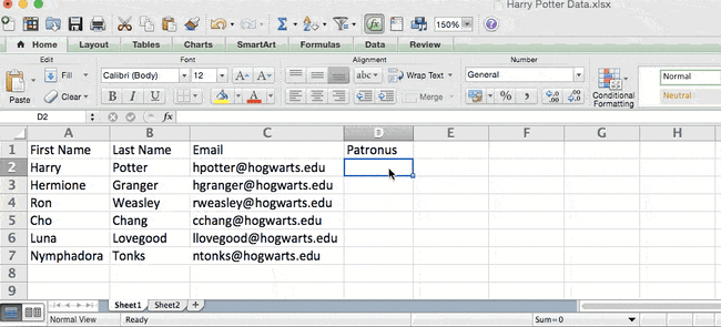
Let‘s have a look at an instance. Let’s say Sheet 1 comprises a listing of individuals‘s names and their Hogwarts electronic mail addresses, and Sheet 2 comprises a listing of individuals’s electronic mail addresses and the Patronus that every pupil has. (For the non-Harry Potter followers on the market, each witch or wizard has an animal guardian referred to as a “Patronus” related to her or him.) The knowledge that lives in each sheets is the column containing electronic mail addresses, however this electronic mail handle column is in several column numbers on every sheet. I‘d use the INDEX and MATCH formulation as a substitute of VLOOKUP so I wouldn’t have to change any columns round.
So what‘s the components, then? The components is definitely the MATCH components nested contained in the INDEX components. You’ll see I differentiated the MATCH components utilizing a special coloration right here.
The components: =INDEX(desk array, MATCH components)
This turns into: =INDEX(desk array, MATCH (lookup_value, lookup_array))
The components with variables from our instance beneath: =INDEX(Sheet2!A:A,(MATCH(Sheet1!C:C,Sheet2!C:C,0)))
Listed here are the variables:
- Desk Array: The vary of columns on Sheet 2 containing the brand new information you wish to convey over to Sheet 1. In our instance, “A” means Column A, which comprises the “Patronus” data for every individual.
- Lookup Worth: That is the column in Sheet 1 that comprises an identical values in each spreadsheets. Within the instance that follows, this implies the “electronic mail” column on Sheet 1, which is Column C. So: Sheet1!C:C.
- Lookup Array: That is the column in Sheet 2 that comprises an identical values in each spreadsheets. Within the instance that follows, this refers back to the “electronic mail” column on Sheet 2, which occurs to even be Column C. So: Sheet2!C:C.
After you have your variables straight, sort within the INDEX and MATCH formulation within the top-most cell of the clean Patronus column on Sheet 1, the place you need the mixed data to dwell.
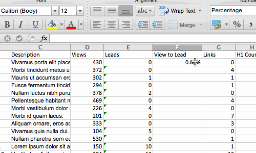
14. Use the COUNTIF perform to make Excel rely phrases or numbers in any vary of cells.
As a substitute of manually counting how typically a sure worth or quantity seems, let Excel do the be just right for you. With the COUNTIF perform, Excel can rely the variety of instances a phrase or quantity seems in any vary of cells.
For instance, to illustrate I wish to rely the variety of instances the phrase “Gryffindor” seems in my information set.
The components: =COUNTIF(vary, standards)
The components with variables from our instance beneath: =COUNTIF(D:D,“Gryffindor”)
On this components, there are a number of variables:
- Vary: The vary that we would like the components to cowl. On this case, since we’re solely specializing in one column, we use “D:D” to point that the primary and final column are each D. If I had been taking a look at columns C and D, I’d use “C:D.”
- Standards: No matter quantity or piece of textual content you need Excel to rely. Solely use citation marks if you’d like the consequence to be textual content as a substitute of a quantity. In our instance, the standards is “Gryffindor.”
Merely typing within the COUNTIF components in any cell and urgent “Enter” will present me what number of instances the phrase “Gryffindor” seems within the dataset.
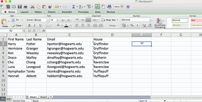
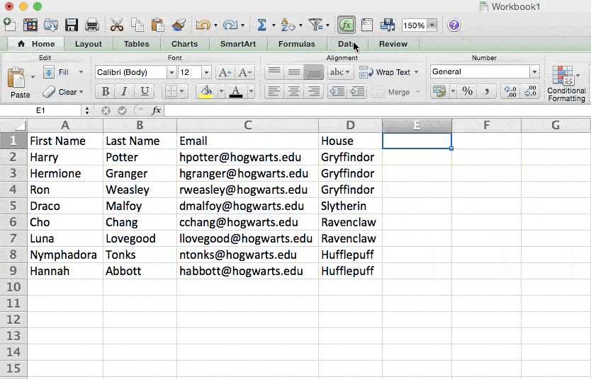
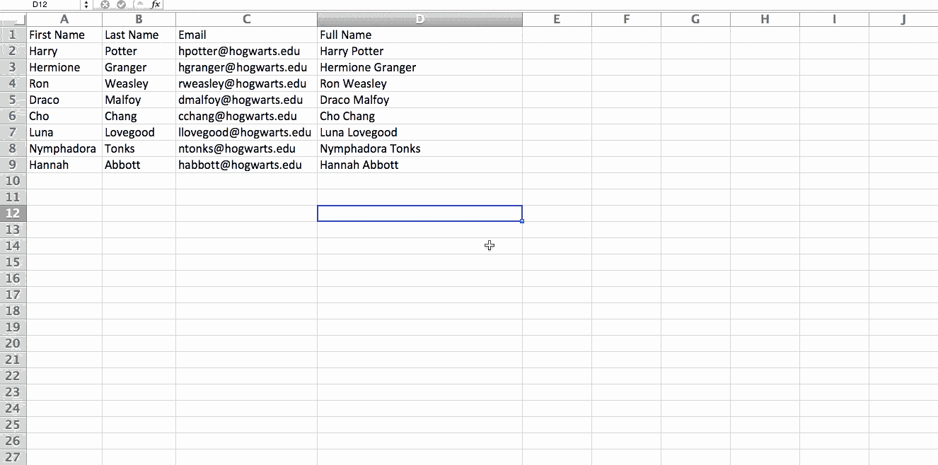
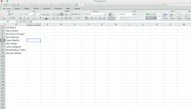
15. Mix cells utilizing &.
Databases have a tendency to separate out information to make it as precise as attainable. For instance, as a substitute of getting a column that reveals an individual‘s full title, a database might need the info as a primary title after which a final title in separate columns. Or, it might have an individual’s location separated by metropolis, state, and zip code. In Excel, you may mix cells with totally different information into one cell through the use of the “&” sign up your perform.
The components with variables from our instance beneath: =A2&“ ”&B2
Let‘s undergo the components collectively utilizing an instance. Fake we wish to mix first names and final names into full names in a single column. To do that, we’d first put our cursor within the clean cell the place we would like the total title to seem. Subsequent, we would spotlight one cell that comprises a primary title, sort in an “&” signal, after which spotlight a cell with the corresponding final title.
However you‘re not completed — if all you sort in is =A2&B2, then there won’t be an area between the individual’s first title and final title. So as to add that essential area, use the perform =A2&“ ”&B2. The citation marks across the area inform Excel to place an area in between the primary and final title.
To make this true for a number of rows, merely drag the nook of that first cell downward as proven within the instance.
16. Add checkboxes.
In the event you‘re utilizing an Excel sheet to trace buyer information and wish to oversee one thing that isn’t quantifiable, you could possibly insert checkboxes right into a column.
For instance, should you‘re utilizing an Excel sheet to handle your gross sales prospects and wish to monitor whether or not you referred to as them within the final quarter, you could possibly have a “Known as this quarter?” column and test off the cells in it while you’ve referred to as the respective shopper.
Here is the right way to do it.
Spotlight a cell you want so as to add checkboxes to in your spreadsheet. Then, click on DEVELOPER. Then, beneath FORM CONTROLS, click on the checkbox or the choice circle highlighted within the picture beneath.
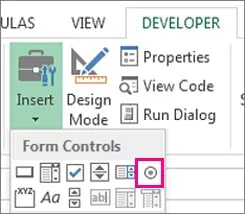
As soon as the field seems within the cell, copy it, spotlight the cells you additionally need it to seem in, after which paste it.
17. Hyperlink a cell to an internet site.
In the event you‘re utilizing your sheet to trace social media or web site metrics, it may be useful to have a reference column with the hyperlinks every row is monitoring. In the event you add a URL immediately into Excel, it ought to routinely be clickable. However, if you must hyperlink phrases, resembling a web page title or the headline of a put up you’re monitoring, here is how.
Spotlight the phrases you wish to hyperlink, then press Shift Ok. From there a field will pop up permitting you to position the hyperlink URL. Copy and paste the URL into this field and hit or click on Enter.
If the important thing shortcut is not working for any purpose, you too can do that manually by highlighting the cell and clicking Insert > Hyperlink.
18. Add drop-down menus.
Typically, you‘ll be utilizing your spreadsheet to trace processes or different qualitative issues. Fairly than writing phrases into your sheet repetitively, resembling “Sure”, “No”, “Buyer Stage”, “Gross sales Lead”, or “Prospect”, you should use dropdown menus to shortly mark descriptive issues about your contacts or no matter you’re monitoring.
Here is the right way to add drop-downs to your cells.
Spotlight the cells you need the drop-downs to be in, then click on the Knowledge menu within the prime navigation and press Validation.
From there, you may see a Knowledge Validation Settings field open. Take a look at the Permit choices, then click on Lists and choose Drop-down Checklist. Examine the In-Cell dropdown button, then press OK.
19. Use the format painter.
As you’ve in all probability seen, Excel has a variety of options to make crunching numbers and analyzing your information fast and simple. However should you ever spent a while formatting a sheet to your liking, you understand it will possibly get a bit tedious.
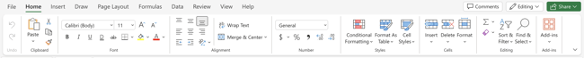
Don’t waste time repeating the identical formatting instructions again and again. Use the format painter to simply copy the formatting from one space of the worksheet to a different. To take action, select the cell you’d like to duplicate, then choose the format painter choice (paintbrush icon) from the highest toolbar.
20. Create tables with information.
Changing your information right into a desk not solely makes it visually interesting but in addition offers improved information administration and evaluation capabilities.
To get began, you’ll want to pick out the vary of cells that you just wish to convert right into a desk. Then, go to the House tab within the Excel ribbon. Within the Kinds group, click on on the Format as Desk button — it seems like a grid of cells. Then, select a desk fashion from the accessible choices, or customise a desk if desired.
Within the Create Desk dialog field, be certain the vary you chose is appropriate. If Excel didn’t routinely detect the vary accurately, you may regulate it manually. In case your desk has headers (column names), make sure that the “My desk has headers” choice is checked. This enables Excel to deal with the primary row because the header row.
As soon as every thing is prepared, click on the OK button, and Excel will convert your chosen information right into a desk.
After your information is transformed right into a desk, you may discover some further options and functionalities turn out to be accessible:
- The desk is routinely assigned a reputation, resembling “Table1” or “Table2,” which you’ll modify if wanted.
- Filter drop-down arrows seem within the header row, permitting you to filter information throughout the desk simply.
- The desk is formatted with alternating row colours, making it visually interesting.
- Complete rows are routinely added on the backside of every column, permitting you to carry out calculations like sum, common, and so on., for the info in that column.
21. Use tables to conduct a what-if evaluation.
Along with making your information extra organized, tables may assist you to conduct what-if analyses. This lets you check numerous combos of enter values and observe the ensuing outcomes.
A what-if evaluation may be helpful relating to determination making, planning, forecasting, monetary modeling, sensitivity evaluation, useful resource planning, and extra.
To get began, you’ll have to arrange your worksheet with the mandatory formulation and variables you wish to analyze. Then, decide the enter values that you just wish to fluctuate. Sometimes, you’ll select one or two enter variables.
Choose the cell the place you wish to show the outcomes of your what-if evaluation. Then, go to the Knowledge tab within the Excel ribbon and click on on the What-If Evaluation button. From the dropdown menu, choose Knowledge Desk.
Within the Desk Enter dialog field, enter the enter values that you just wish to check for every variable. If in case you have one variable, enter the totally different enter values in a column or row. If in case you have two variables, enter the combos in a desk format.
Choose the cells within the desk space that correspond to the components cell you wish to analyze. That is the cell that may show the outcomes for every mixture of enter values.
Click on OK to generate the info desk. Excel will calculate the components for every mixture of enter values and show the leads to the chosen cells. The information desk acts as a grid, exhibiting the varied eventualities and their corresponding outcomes.
As soon as your desk is created, you should use it to establish traits, patterns, or particular values of curiosity. Mess around with the enter values and see the way it could have an effect on the ultimate outcomes.
22. Make formulation simpler to grasp with named ranges.
As a substitute of referring to a variety of cells by its coordinates (e.g., A1:B10), you may assign a reputation to it. This makes formulation extra readable and simpler to handle.
To get began, choose the cell or vary of cells that you just wish to title. Go to the Formulation tab within the Excel ribbon and click on on the Outline Title button within the Outlined Names group. Alternatively, you should use the keyboard shortcut Alt + M + N + D.
Within the New Title dialog field, enter a reputation for the chosen cell or vary within the Title area. Be certain that the title is descriptive and simple to recollect. By default, Excel assigns the chosen cell or vary’s reference to the Refers to area within the dialog field. If wanted, you may modify the reference to incorporate further cells or regulate the vary.
Click on the OK button to save lots of the named vary. As soon as you have named a variety, you should use it in your formulation by merely typing the title as a substitute of the cell reference. For instance, should you named cell A1 as “Income,” you could possibly use =Income as a substitute of =A1 in your formulation.
Utilizing named ranges gives a number of advantages:
- Improved components readability: Named ranges make formulation simpler to grasp and navigate, particularly in advanced calculations or giant datasets.
- Flexibility for vary changes: In case your dataset adjustments, you may simply modify the vary assigned to a named vary with out updating every components that references it.
- Enhanced collaboration: Named ranges make it simpler to collaborate with others, as they’ll perceive the aim of a named vary and use it in their very own calculations.
- Simplified information evaluation: When utilizing named ranges, you may create extra intuitive information evaluation by referring to named ranges in capabilities like SUM, AVERAGE, COUNTIF, and so on.
To handle named ranges, you may go to the Formulation tab, click on on the Title Supervisor button within the Outlined Names group. The Title Supervisor gives functionalities to switch, delete, or evaluate present named ranges.
23. Group information to enhance group.
Grouping information in Excel offers a technique to manage, analyze, and current data extra successfully, making it simpler to establish patterns, traits, and insights inside your information. For example, you probably have a listing of leads generated, you may group the info by month to create a month-to-month efficiency report.
Grouping information particularly makes it simpler to navigate and work with giant information units. It helps in group and reduces muddle by collapsing the teams that aren’t instantly wanted.
To group information in Excel, choose the vary of cells or columns that you just wish to group. Be certain that the info is sorted correctly, if wanted.
On the Knowledge tab within the Excel ribbon, click on on the Group button. It’s normally discovered within the Define or Knowledge Instruments group.

You possibly can specify the grouping ranges by selecting choices like Rows or Columns. For instance, if you wish to group information by month, you may choose Months. You can too set further choices resembling Abstract rows beneath element or Collapse the define to the abstract ranges. These choices have an effect on how the grouped information is displayed.
After you have the choices you need chosen, click on on the OK button, and Excel will group the chosen information based mostly in your settings.
After your information is grouped, you will note a plus (+) or minus (-) button subsequent to the grouped rows or columns. Clicking on the plus button expands the group to indicate the person data, and clicking on the minus button collapses the group to cover the small print.
24. Use Discover & Choose to streamline formatting.
Why format and clear up your spreadsheet manually when you are able to do it in only a few clicks? Utilizing the Discover & Choose software will help you keep accuracy and consistency in your paperwork.
To get began, open the Excel worksheet that comprises the info you wish to search. Press the Ctrl + F keys in your keyboard or go to the House tab and click on on the Discover & Choose drop-down menu. Then, choose Discover from the menu. The Discover and Change dialog field will open.
Within the Discover area, enter the particular information you wish to discover. Optionally, you may slender down your search to particular cells, rows, columns, or formulation by selecting the suitable choices within the dialog field.
Click on on the Discover subsequent button to seek for the primary prevalence of the info. Excel will spotlight the cell containing the info.
To exchange the discovered information with new data, click on on the Change button within the dialog field. It will change the highlighted prevalence with the info you enter within the Change area.
To exchange all occurrences of the info directly, click on on the Change All button. After you have completed discovering and changing, you may shut the dialog field.
Observe: Be cautious when utilizing the Change All characteristic, because it replaces all occurrences with out affirmation. It’s all the time a great follow to evaluate every alternative fastidiously earlier than utilizing the Change All choice.
25. Defend your work.
Defending your work in Excel is crucial for information safety, sustaining information integrity, preserving mental property, and complying with authorized or regulatory necessities. It lets you have management over who can entry and modify your work, minimizing dangers and sustaining the standard and confidentiality of your information.
Listed here are a pair methods you may defend your work:
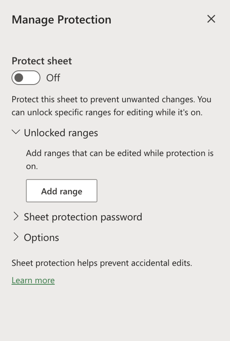
Defend a Worksheet
- Open your Excel worksheet and navigate to the Evaluate tab.
- Click on on the Handle Safety button within the Safety group.
- A Handle Safety dialog field will seem. There, you may choose whether or not or not you wish to defend the sheet. Set a password if desired and select the choices you wish to apply, resembling stopping customers from making adjustments to cells, formatting, inserting/deleting columns or rows, and so on.
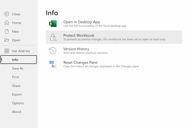
Defending a Workbook
- Open your Excel workbook and navigate to the File tab.
- Click on on Data and choose Defend Workbook from the choices.
- Select Encrypt with Password and enter a password if desired.
- Click on OK to guard the workbook.
Taking these further steps ensures your work is protected. Simply be certain to maintain your passwords protected and safe.
26. Create customized quantity codecs.
To show information in distinctive methods, use customized quantity codecs. Doing this will help with information presentation, information readability, consistency, localization, and masking delicate information.
To get began, choose the cell or vary of cells that you just wish to format. Proper-click on the chosen cells and select Quantity Format from the context menu. Then, discover the Class listing and choose Customized.
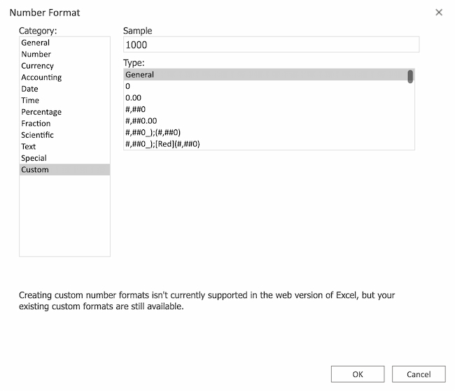
Within the Sort area, you may enter a customized quantity format code to outline your required format. Listed here are some examples of customized quantity codecs:
- To show numbers with a selected variety of decimal locations, use the 0 or # image to characterize a digit, and a zero or hashtag with out a decimal level to characterize non-obligatory digits. For instance, 0.00 will show two decimal locations, 0.### will show as much as three decimal locations, and ### will show no decimal locations.
- To show a selected textual content or character alongside numbers, use the @ image. For instance, $0 will show a greenback signal earlier than the quantity.
- To show percentages, use the % image. For instance, 0% will show the quantity as a proportion.
- To create customized date or time codecs, use codes resembling dd for day, mm for month, yy for two-digit yr, hh for hours, mm for minutes, and ss for seconds. For instance, dd/mm/yyyy will show the date within the format of day/month/yr.
As you enter your customized quantity format within the Sort area, you will note a Pattern part that reveals a preview of how the format will likely be utilized. Click on OK to use the customized quantity format to the chosen cells.
27. Customise the Excel ribbon.
Though the Excel ribbon already comprises numerous instruments which can be used to execute widespread capabilities and instructions, you may customise it to suit your particular wants and preferences.
This will help streamline your workflow and make generally used instructions extra simply accessible. It additionally lets you take away pointless parts that you just don’t use, making it simpler to navigate and discover the instruments you want.
To make customizations, begin by proper clicking on an empty space of the ribbon and choose Customise the Ribbon. Within the Excel Choices window that seems, you may see two sections. The left part shows the tabs at the moment seen within the ribbon, whereas the best part shows the tabs you may add.
To customise the ribbon, you may have a number of choices:
- So as to add a brand new tab, click on on New Tab in the best part and provides it a reputation.
- So as to add a bunch inside an present tab, choose the tab within the left part, click on New Group in the best part, and title it.
- So as to add instructions to a bunch, choose the group in the best part, select instructions from the left part, and click on Add. You can too customise the order of the instructions utilizing the Up and Down buttons.
You can too take away tabs, teams, or instructions from the ribbon. Choose the merchandise you wish to take away within the left part and click on Take away.
To alter the order of tabs and teams, choose the merchandise within the left part and use the Up and Down buttons to rearrange them.
Click on OK within the Excel Choices window to save lots of your adjustments and apply the custom-made ribbon.
To increase Excel’s performance even additional, you may customise the ribbon with further purposes by clicking on the Add-ins button within the House tab.
Observe: Customizing the ribbon is restricted to your Excel set up and gained‘t have an effect on different customers’ ribbons.
28. Enhance visible presentation with textual content wrapping.
Although spreadsheets aren’t all the time essentially the most attention-grabbing issues to take a look at, you may nonetheless take the time to make them simpler to learn by wrapping textual content.
Doing this allows you to show a number of traces of textual content inside a single cell. It is notably helpful when you should embrace line breaks or break up paragraphs of knowledge inside a cell with out growing the row peak.
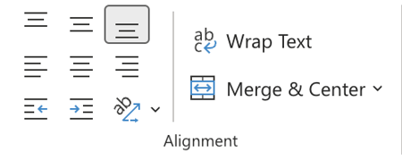
Choose the cell(s) with the textual content you wish to wrap. Navigate to the toolbar on the prime of the Excel window and find the Wrap Textual content button (an icon with an angled arrow). It’s sometimes discovered within the Alignment part. Then, click on on Wrap Textual content.
29. Add emojis.
Give your spreadsheets a bit private contact by including in emojis.
To get began, click on on the cell the place you wish to insert an emoji. Then, open the emoji keyboard. This step could fluctuate based mostly in your working system.
- Home windows: Use the keyboard shortcut Win + . or Win + ; to open the emoji keyboard.
- macOS: Use the keyboard shortcut Ctrl + Cmd + House to entry the emoji keyboard.
Flick through the accessible emojis and click on on the one you wish to insert. The chosen emoji ought to now seem within the chosen cell.

Emojis could seem small by default in Excel cells. If you wish to make them bigger to enhance visibility, you may regulate the cell measurement by dragging the row peak and column width accordingly.
You can too copy emojis from exterior sources on the net or different purposes and paste them immediately into Excel cells.
Observe: The flexibility to make use of emojis in Excel is determined by the model of Excel and the system you might be utilizing. Some older variations or platforms could not help emojis or show them accurately. Subsequently, it is vital to make sure compatibility with the Excel model and platform you might be working with.
Excel Keyboard Shortcuts
Creating studies in Excel is time-consuming sufficient. How can we spend much less time navigating, formatting, and deciding on gadgets in our spreadsheet? Glad you requested. There are a ton of Excel shortcuts on the market, together with a few of our favorites listed beneath.
Create a New Workbook
PC: Ctrl-N | Mac: Command-N
Choose Total Row
PC: Shift-House | Mac: Shift-House
Choose Total Column
PC: Ctrl-House | Mac: Management-House
Choose Remainder of Column
PC: Ctrl-Shift-Down/Up | Mac: Command-Shift-Down/Up
Choose Remainder of Row
PC: Ctrl-Shift-Proper/Left | Mac: Command-Shift-Proper/Left
Add Hyperlink
PC: Ctrl-Ok | Mac: Command-Ok
Open Format Cells Window
PC: Ctrl-1 | Mac: Command-1
Autosum Chosen Cells
PC: Alt-= | Mac: Command-Shift-T
Different Excel Assist Sources
Use Excel to Automate Processes in Your Crew
Even should you’re not an accountant, you may nonetheless use Excel to automate duties and processes in your workforce. With the ideas and tips we shared on this put up, you’ll make sure you use Excel to its fullest extent and get essentially the most out of the software program to develop your enterprise.
Editor’s Observe: This put up was initially printed in August 2017 however has been up to date for comprehensiveness.
